PID Controller basics

The PID controller is the most commonly used controller in the praxis and it becomes the standard tool when process control emerges in the 1940s. More than 90% of the control loops today are passed on the PID controller and especially PI control.

PID controller basics

Generally the controller combines: sensors, controllers, actuators. The PID controller is the most common controller, it is a simple three-term controller. The letters P, I and D stand for:

• P roportional
• I ntegral
• D erivative

This principle mode of action of the PID controller can be explained by the parallel connection of the P, I and D elements shown in Figure 1

In this article we assume that the controller is used in a closed-loop unity feedback system. Consider a system for automatic control consisting of an object Wo(p) and regulator Wp(p). The names of the signals in the system: y - output value of the object, r – setpoint (reference variable), e - error (e = r - y), u - control signal.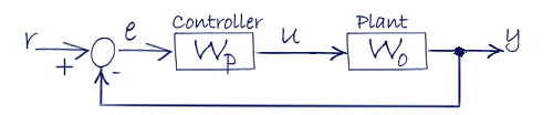

Figure 1.

The control signal u from the controller to the plant changed in the time: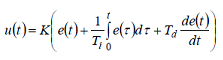

Equation 1.

Equation 1 represents the ideal PID controller. The control signal u(t) is the sum of the three components: P-term (proportional to the error), I-term (proportional to the integral of the error) and D-term (proportional to the derivative of the error), where e(t) is the error.
The controller parameters are the gain K, time constant of the integration Ti and derivative time Td. Integral, proportional and derivative components can be interpreted as managing impacts based on past, present and future.
τ (tau) is the variable of integration.

This control signal u is fed to the plant and the new output y is obtained and compared to the reference to find the new error signal e. The controller takes this new error signal and computes an update of the control input.

PID Controller representation

The PID algorithm in Equation 1 is seldom used. So there are some other ways in representing the PID controller.
The transfer function of a PID controller can be found by taking the Laplace transform of Equation 1.

Equation 2.

Equation 2 gives us the parallel representation of the PID controller.

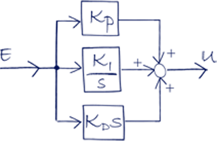
Figure 2. PID parallel representation.

Second way of representing the PID controller is the standard representation.

Equation 3.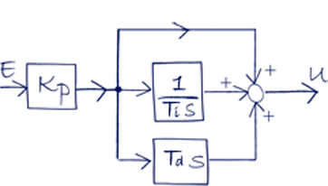

Figure 3. PID standard representation.

And the third way of representing the PID controller is the classical/serial method.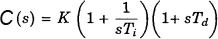

Equation 4.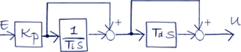

Figure 4. PID seria/classicall representation.

The three forms are mathematically equivalent. The main difference between those structures is the effects of setting coefficients on the controller’s behavior. The parallel form for example allows for a complete decoupling of proportional, integral and derivative actions whereas with a standard structure a modification of the Kp coefficient will affect proportional, integral and derivative actions.
Another example if you set the derivative part in the standard and in the classical representation to 0 you will notice they are identical.

Before start tuning the controller you have to be sure which type is used. Some distributers use different abbreviations in their manuals but the structure of the equations is always the same, so that will tell you what type you have.

 

The Transfer function of a system is the relationship of the system's output to its input.

 

PID components

Proportional component

The proportional component depends only on the difference between the set point and the process variable. The proportional gain determines the ratio of output response to the error signal.
Increasing the proportional gain will increase the speed of the control system response. But if the proportional gain is too large, the process variable will begin to oscillate the system may become unstable and oscillate out of control.
Working only with proportional control will result in an error between the setpoint and the actual process value, because non-zero error is required to drive it, the so called steady state error (SSE). If there is no error, there is no corrective response.

Integral component

The integral component sums the error over its duration. The integral response will continually increase over time unless the error is zero, so the goal is to bring the Steady-State error to zero.
By decreasing the integral time Ti we can increase the influence of the integral component, the disadvantage here is that when decreasing Ti the tendency of oscillations will increase, the controller output overshoots.

Derivative component

The derivative mode provides an output that is proportional to the rate of change of the error with respect to time. It also makes the loop more stable (up to a point) which allows using a higher controller gain and a faster integral (shorter integral time or higher integral gain).
Increasing the derivative time (Td) parameter will cause the control system to react more strongly to changes in the error term and will increase the speed of the overall control system response.
Most practical control systems use very small or none derivative component, because the Derivative Response is highly sensitive to noise in the process variable signal. If the sensor feedback signal is noisy or if the control loop rate is too slow, the derivative response can make the control system unstable.

System characteristics

When designing a control system we have to know the system which is to be controlled, we need to identify its characteristics. By putting energy to the system we can analyze the response of it in order to understand the system dynamics.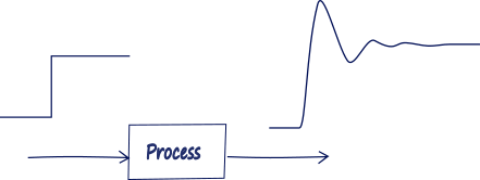

Figure 5.

Four major characteristics of the system step response are shown below on Figure 6: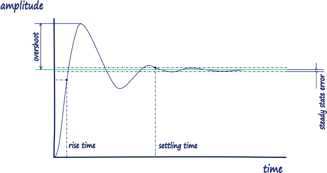

Figure 6.

Rise Time, the time it takes for the plant output y to rise beyond 90% of the desired level for the first time.
Overshoot, how much the peak level is higher than the steady state, normalized against the steady state.
Settling Time, the time it takes for the system to converge to its steady state.
Steady-state Error, the difference between the steady-state output and the desired output.
And this is how increasing each of the PID parameters affects these four characteristics:

P - Proportional

• Rise Time: Decrease
• Overshoot: Increase
• Settling time: Almost not affected
• Error: Decrease
  
  

I – Integral

• Rise Time: Decrease
• Overshoot: Increase
• Settling time: Increase
• Error: Eliminate
  
  

D – Derivative

• Rise Time: Almost not affected
• Overshoot: Decrease
• Settling time: Decrease
• Error: Almost not affected

Basically summarized while tuning PID controller we will use the P-term to decrease the Rise Time, I-term to eliminate the steady state error, D-term to reduce the overshoot and settling time